
Appearance
Geometry and spatial indices
Five layers whose shape comes from the data rather than from a coordinate pair: an explicit geometry, and four global grids addressed by identifier.
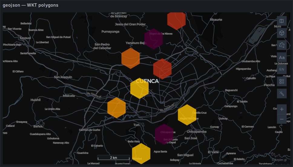
geojson
sql
SELECT geom, name, value, zona
FROM neighbourhoods;
Polygons, lines and points from a geometry column. Built automatically — the panel renames the column to kepler's _geojson and kepler creates the layer.
The column can hold GeoJSON, WKT, or raw WKB/EWKB hex; the image above is WKT. WKB decoding happens in the plugin, which is what lets a plain SELECT geom from PostGIS render with no ST_AsGeoJSON around it. See Geometry.
Fill and stroke are separately controllable, and polygons can be extruded into 3D by a column with the 3D control on.
Cost: the only layer here whose weight is unrelated to its row count. A hundred detailed municipal boundaries can outweigh a million points. Simplify in the query — ST_Simplify(geom, 0.0005) — rather than hoping the browser copes.
Backed by deck.gl's GeoJsonLayer.
h3
sql
SELECT h3_index AS h3, COUNT(*) AS value, zona
FROM readings
GROUP BY 1, 3;
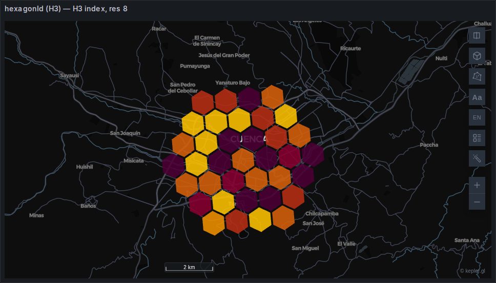
Uber's hexagonal grid. The index is the geometry: the layer derives each hexagon's boundary from the identifier, and the resolution comes from the index itself, so nothing needs configuring.
Built automatically, and by a mechanism worth knowing: kepler types a string column as H3 when its values are valid H3 cells, so detection is by content rather than by name. A column of good indices produces a layer under any name.
Distinct from the hexagon layer, which bins raw points in the browser. This one draws cells your data already carries — which means the aggregation happened in SQL, where it is far cheaper.
Backed by deck.gl's H3HexagonLayer, plus ColumnLayer when extruded.
s2
sql
SELECT s2_token AS s2, COUNT(*) AS value, zona
FROM sightings
GROUP BY 1, 3;
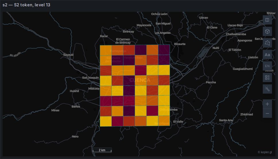
Google's quadrilateral grid, addressed by token. The same idea as H3 with square cells.
S2 is detected by name, not by value
There is no S2 role in Field mapping, and kepler's own detection looks for a column named exactly s2 or s2_token. A column called anything else produces no layer.
The gallery panel above is an illustration of this: its column is called token, so the layer is not autodetected at all — it is pinned by a saved map configuration. In your own dashboard, alias the column to s2 and it works without one.
Backed by deck.gl's S2Layer.
geohash
sql
SELECT geohash, count(*) AS readings
FROM readings
GROUP BY geohash;
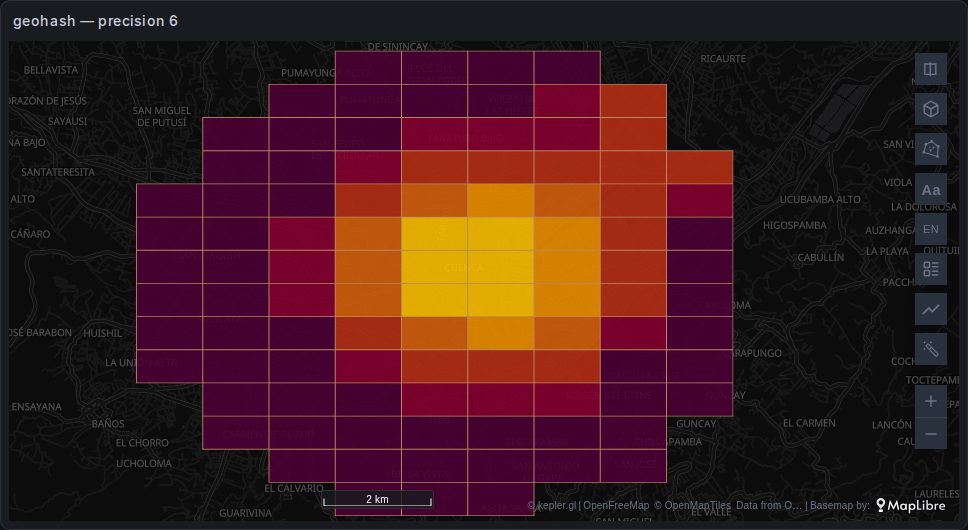
The rectangles of the geohash grid. Each cell is drawn from its identifier, and the identifier's length is its precision: the cells above have six characters, about 1.2 by 0.6 km.
Built automatically. kepler creates a GeoHash layer for a column named geohash, geo_hash or geohash_id. The panel reads a column named geohash as well, or the one chosen in Field mapping → Geohash, and places each row at the centre of its cell when the query has no latitude and longitude of its own (see Places by geohash or by name). Such a query then gets one GeoHash layer, the panel's, in place of kepler's GeoHash and a Point layer of dots on the centres. The centres stay in the dataset: a Point or Heatmap layer added by hand draws them, and click variables read them.
| Column | Cells | Centres |
|---|---|---|
geohash | yes | yes |
geo_hash, geohash_id | yes | no |
| any other, chosen in Field mapping → Geohash | yes | yes |
A query with coordinates of its own keeps them: there, a geohash column gets kepler's GeoHash layer beside the Point layer on the query's coordinates.
A value must be text of 1 to 12 characters from the geohash alphabet; case does not matter. Rows whose value is not a geohash are left out of the layer.
In the layer's panel: fill colour by a column, outline colour and width by a column, and height by a column with the 3D control on.
Backed by deck.gl's GeohashLayer.
a5
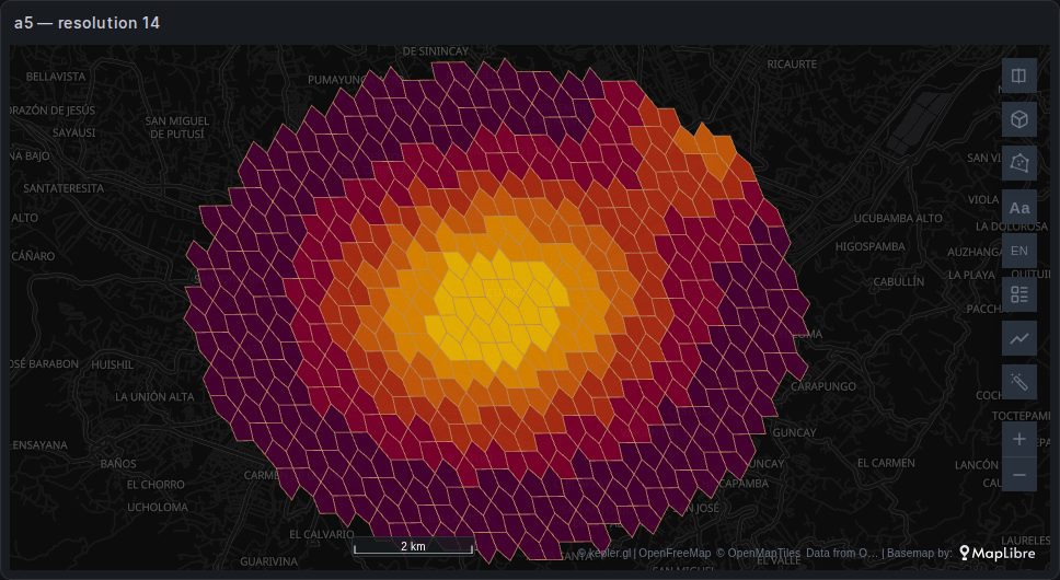
sql
-- DuckDB, with the a5 extension loaded
SELECT a5_u64_to_hex(a5_lonlat_to_cell(lon, lat, 14)) AS a5, count(*) AS readings
FROM readings
GROUP BY 1;
A5 is a global grid of pentagons. Like H3 and S2, the cell identifier is the geometry and carries its own resolution, 0 to 30.
Built automatically by kepler for a column named a5, a5_token or a5_id. There is no A5 role in Field mapping: alias the column to one of those names, or add the layer by hand from Add Layer → A5 and point its column at yours.
Send the cell as hexadecimal text
An A5 cell is a 64-bit integer, and a JavaScript number holds integers exactly only up to 2⁵³. kepler accepts a number only below that limit, and cells lie far above it: the one at the centre of the image is about 3 × 10¹⁸. A query that returns the cell as an unsigned 64-bit number still gets an A5 layer, and it draws nothing. Return the cell as its hexadecimal string instead — a5_u64_to_hex in DuckDB — as the query above does.
The controls are the same as GeoHash's. kepler ships no name for this layer type; the panel names it A5 in the layer list.
Backed by deck.gl's A5Layer.
Choosing between them
| Your data is | Use |
|---|---|
| Real boundaries — administrative, parcels, routes | geojson |
| Already aggregated to H3 cells | h3 |
| Already aggregated to S2 cells | s2 |
| Already aggregated to geohashes | geohash |
| Already aggregated to A5 cells | a5 |
| Raw points you want binned | hexagon or grid |
Between H3 and S2, prefer H3 if you have a choice: it is a panel role, it is detected from values rather than names, and it works for origin–destination flows. Use S2 when your data already arrives that way.