Points and aggregation

Twelve ways to read the same rows. Every image on this page but the Cells and Donut ones comes from a single query returning latitude, longitude, a numeric value and a categorical zona — the difference is entirely in which layer you point at it.

SELECT lat AS latitude,
       lon AS longitude,
       value,
       zona
FROM readings;

Only the first is built for you. The others you add in kepler's layer panel: + Add Layer, pick the type, pick the dataset.

point

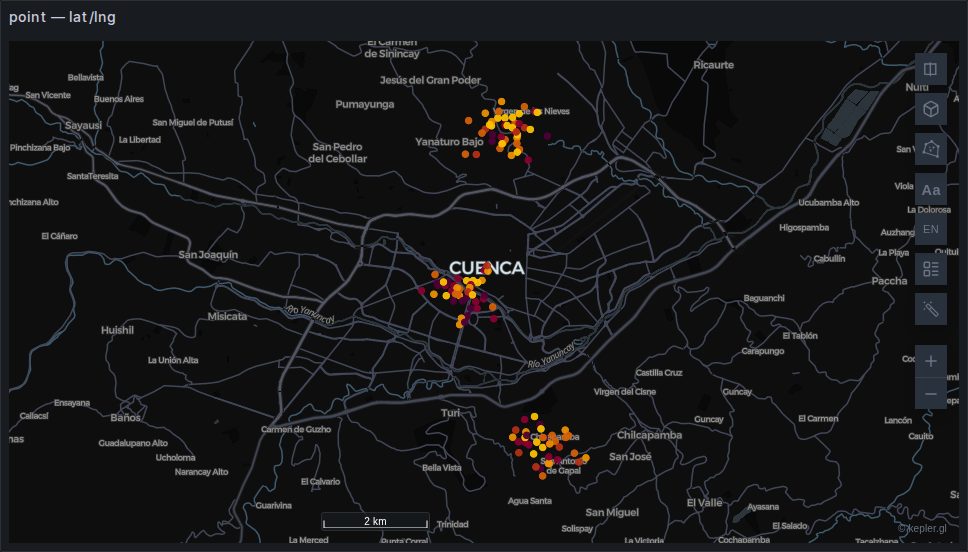
One circle per row. Colour and radius can each be driven by a column, which is usually enough to read a dataset before reaching for anything cleverer.

Built automatically from a latitude/longitude pair. Backed by deck.gl's ScatterplotLayer and the cheapest thing on this page — hundreds of thousands of rows is comfortable.

TIP

The default radius is small. On a country-sized view a few thousand points can look like an empty map; raise Radius before concluding nothing rendered.

Two effects under Visual, both off by default:

• Glow puts a soft halo round each point: Extent is its radius as a multiple of the point's (2 by default), Strength how bright it is.
• Pulse / Ripple animates each point: Pulse swells and shrinks it, Ripple sends a ring out from it, at Speed cycles a second and out to Expansion times its radius. With Trigger set to Continuous every point pulses all the time; with At event time a point pulses when the end of the map's time window reaches the time in its Event timestamp column, and for Duration of timeline time after it. That needs an enabled time filter on the same column: the one Time range sync puts on the map is one, as is one added in kepler's filter panel; without it the layer panel says what is missing. The pulses follow the window as it plays or is dragged, which makes events stand out: earthquakes, alarms, sales.

heatmap

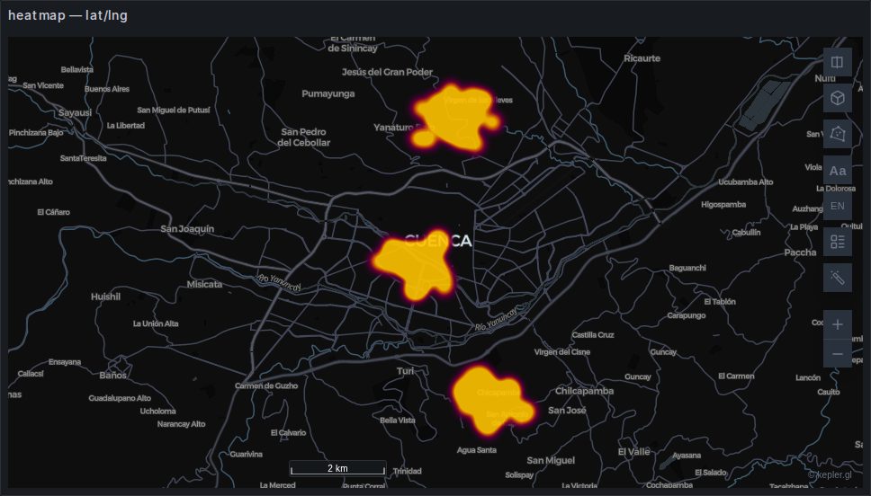
A continuous density surface. Good for "where is the concentration", useless for "how many" — there is no legend that makes a heatmap quantitative, and the apparent intensity changes with zoom.

Weight can be driven by a column; left alone it counts rows.

3D Surface lifts the heatmap into a relief whose height is the density, up to Maximum height in metres; tilt the map to see it. Surface shading lights it, and Surface contours draws lines across it every Contour step of density. The height is density, not terrain: it does not follow the base map's relief.

Backed by deck.gl's HeatmapLayer from @deck.gl/aggregation-layers; the surface is a mesh kepler builds from the same density.

contour

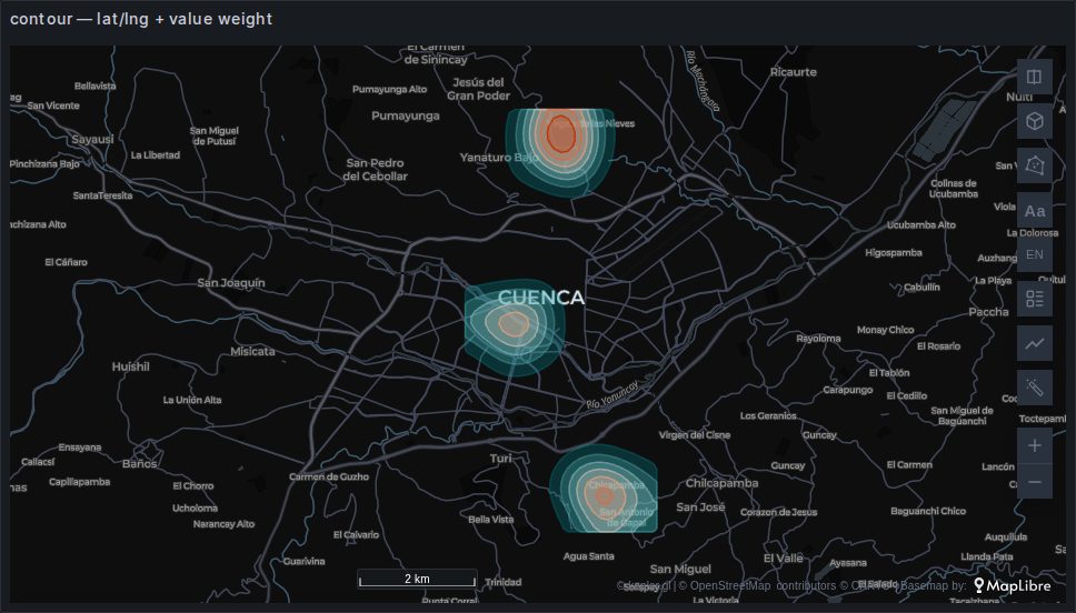
Lines of equal density, the way a topographic map draws equal height. The points are counted into a grid, smoothed, and traced at a number of levels, each band filled in a colour of its own; the legend lists the levels. Where a heatmap only says "more here", a contour says "at least this much inside this line" — hover a band and it reads, for instance, value ≥ 12.

• Weight: a numeric column, averaged within each cell. Left empty, the contours are of the number of points per cell.
• Number of levels (7), Grid resolution (cells along the longer side of the data, 64) and Smoothing (in cells, 3) shape the lines: more cells follow the points closely, more smoothing rounds them off.
• Fill below each level turns the bands inside out, to enclose the lows instead of the peaks. Custom level range sets the lowest and highest level yourself, so two maps can share them.
• Fill, Color by level, Opacity of the fill and Outline width. Custom outline color gives the lines a colour of their own, apart from the fill's.
• 3D surface drapes the fills and outlines over the smoothed surface, raised by Elevation multiplier: at 1× the relief from the lowest to the highest value is a tenth of the grid's longest side. The levels stay in the data's units. Tilt the map to see it.

It takes a latitude/longitude pair or a GeoJSON column (the centre of each shape). New in kepler.gl 3.3.0-alpha.20, its 3D surface and outline colour in 3.3.0-alpha.21. The contours are computed in the browser, again with every filter change; keep the rows to tens of thousands.

Backed by deck.gl's GeoJsonLayer.

grid

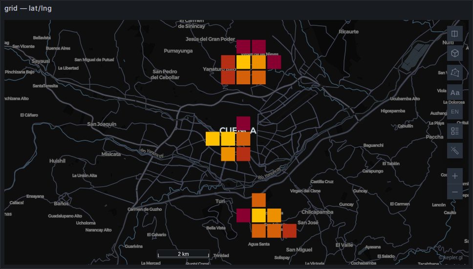
Square bins, sized in metres by Grid Size. Unlike a heatmap it is quantitative: each cell has a value you can colour and extrude, and a legend that means something.

Extrusion turns it into a 3D histogram, which needs the 3D control and reads best with a lighting effect turned on.

Backed by deck.gl's GridLayer.

hexagon

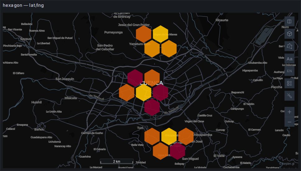
The same idea with hexagonal bins. Hexagons have a single distance to all six neighbours, which avoids the diagonal artefacts a square grid produces on clustered data — the reason most people prefer them for movement data.

Coverage shrinks each hexagon within its cell, which is how you get the gaps between them.

Backed by deck.gl's HexagonLayer. Distinct from the H3 layer: this bins raw points in the browser, while hexagonId draws cells your data already carries.

cells

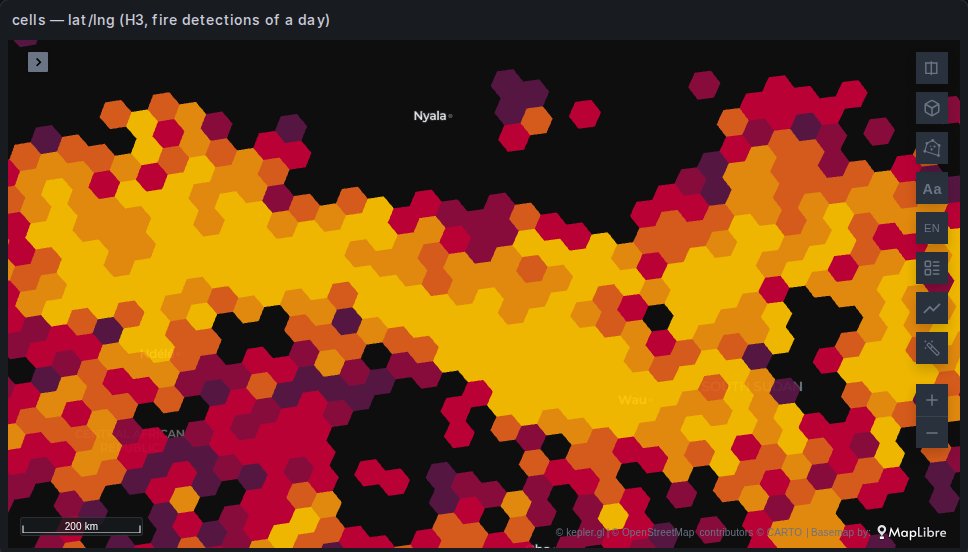
Since 1.8.0

The cells layer is new in 1.8.0.

Points counted in the cells of a global grid, H3, A5, S2 or geohash, at the level that suits the zoom: each cell is about Cell size pixels across, so the map refines as you zoom in and coarsens as you zoom out, where a hexagon layer keeps its radius in kilometres at every zoom. A layer type this plugin adds, named Cells, built on kepler's hexagon layer: the colour and height channels, Count, Sum, Average and the other aggregations, the legend, the popup, the count labels and the filters are the hexagon layer's.

• Cell system picks the grid. A5 and S2 split each cell in four, so their level changes once per zoom level; H3 splits in seven, every 1.4 zoom levels or so, and geohash in 32, every 2.5, with bigger jumps. A5's cells all have the same area, H3's and S2's vary by about two times between places, and geohash's shrink towards the poles.
• Cell size (in the Radius group, where the hexagon layer has its radius) is how many pixels across a cell should be; the level is the one closest to it.
• Per km² divides each cell's value by its area, so a colour means the same density at every zoom and latitude.
• Transition eases the cells to their new colours and heights when the level changes, a filter moves or the data refreshes: zooming in, the new cells come out of their parent's colour; zooming out, a cell starts from the mean of its children's. 0 switches it off.
• The colours are those of the cells around the view, not of the whole dataset, so the legend is the view's: zoomed in on a dense region, its cells spread over every class instead of all landing in the top one. Panning far recolours.
• Color Scale adds Log and Sqrt to the hexagon layer's scales: classes evenly spaced on that axis, which suits counts running from one to thousands per cell.

Each point is placed once, at a fine level, and every coarser cell is its parent, so a zoom costs little. Placing is the slow part for A5, about 25,000 points a second; H3, S2 and geohash place hundreds of thousands. Cells far outside the view are not drawn until you pan towards them.

Unlike hexagonId and the other index layers, this one takes points: the cells are worked out in the browser. With more rows than the browser should receive, count in SQL instead and draw the cells with those layers.

Backed by deck.gl's H3HexagonLayer, A5Layer, S2Layer and GeohashLayer.

cluster

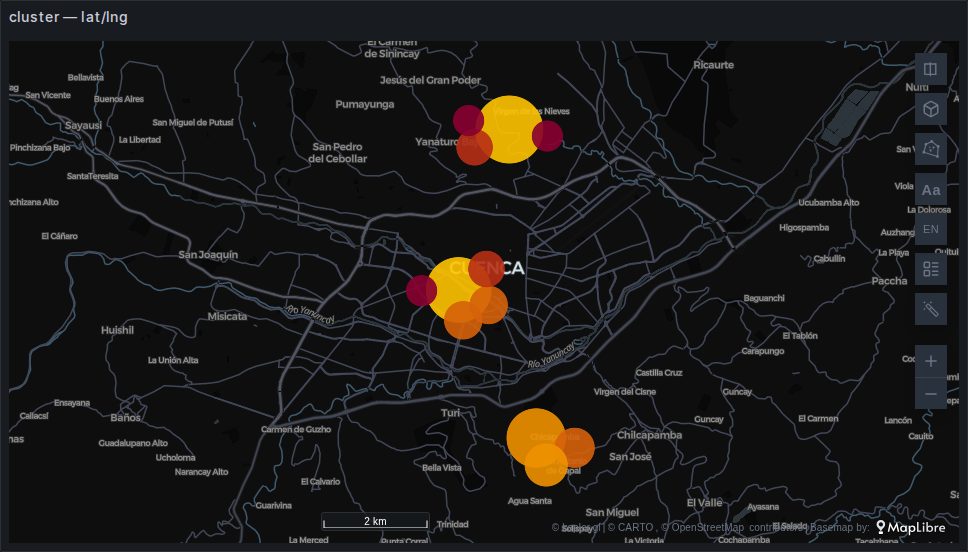
Points grouped into circles sized by how many they contain, re-clustered as you zoom. The familiar "47" bubble from web maps.

Better than a heatmap when the count matters and better than raw points when they overlap, but note that the clusters are a rendering artefact — they change as you zoom, so they are not a stable unit to compare.

Backed by a kepler CompositeLayer over deck.gl's ScatterplotLayer.

voronoi

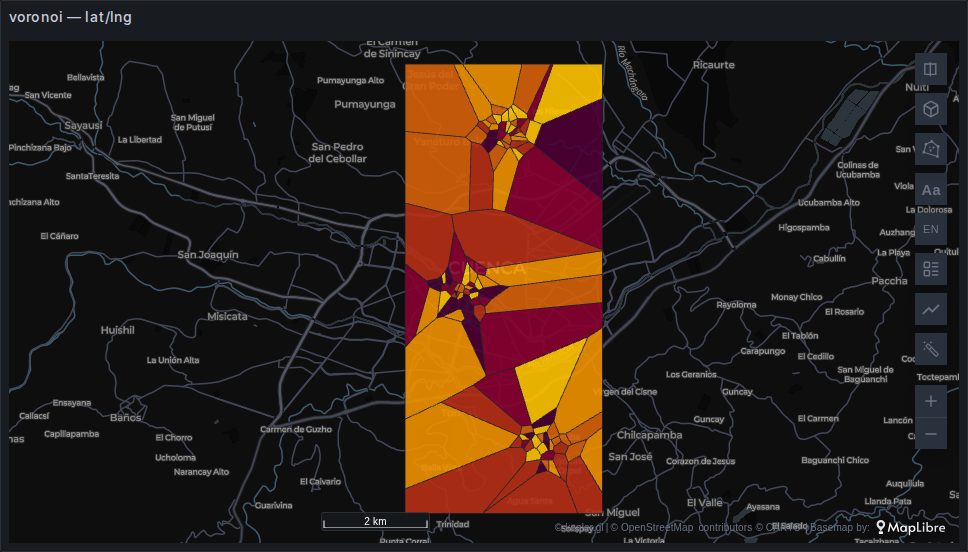
Voronoi Mosaic in the layer menu. Each point gets the part of the map that is nearer to it than to any other point, so every place on the map takes the colour of its nearest point: stations becoming the areas they stand for, without interpolating between them. Colour it by a column as you would a point layer; the cells have an outline, dark by default.

The cells stop at the data's bounding box, widened on each side by Bounds Padding (10 % by default). Nearness is measured on the map, not along streets: a cell is not a catchment area.

It takes a latitude/longitude pair or a GeoJSON column (the centre of each shape). New in kepler.gl 3.3.0-alpha.20, never built for you; switching a point layer's type to it keeps its columns.

Backed by deck.gl's PolygonLayer, the cells computed in the browser with d3-delaunay.

donut

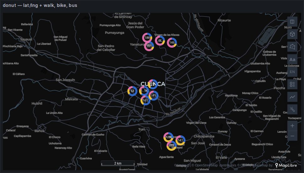
A ring at each point, split into the shares of up to six numeric columns that are parts of one whole: trips by mode, votes by party, a building's energy by source. Pick the columns under Composition, each with its own colour and label; with one column the ring is filled in its colour. Show total in center writes the sum of the columns inside the ring.

Near points are grouped as you zoom out, within Cluster radius pixels of each other: the columns are summed before the shares are taken, so a group's ring is the mix of all its points, and filters apply before the grouping. Radius is the ring's size in pixels. Hover a ring for each column's value and share, the total and how many points it groups.

The columns must be zero or more: a missing value counts as zero, a negative one is left out and counted in the tooltip, and a ring whose total is zero is not drawn. Colour comes from the columns, so there is no colour channel to set.

It takes a latitude/longitude pair. New in kepler.gl 3.3.0-alpha.21, never built for you. The gallery's map is the same points as the others with three columns, walk, bike and bus, mixed differently in each zona.

Backed by deck.gl's ScatterplotLayer drawn as rings, and a TextLayer for the totals.

icon

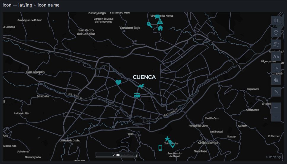
A symbol per row, chosen per row by a column holding an icon name.

SELECT lat AS latitude, lon AS longitude, icon, zona
FROM stations;

The icon library ships with the plugin rather than being fetched from a CDN, which is what makes this work on an air-gapped install and under a strict connect-src. The names are kepler's own; the picker in the layer panel lists them.

Useful for a small number of meaningful things — stations, incidents, depots. At a few hundred rows it becomes noise.

An angle column turns each icon by its own number of degrees, counter-clockwise (since kepler.gl 3.3.0-alpha.20). A compass bearing runs clockwise from north, so pass 360 - heading, or use the symbol layer, which reads a bearing as it is.

symbol

A symbol per row, turned and sized by columns. Its Draw selector picks what each symbol is:

• A shape: one of about a thousand map symbols — the plugin's own shapes, Maki, Temaki and the UN OCHA humanitarian icons (named temaki:… and ocha:…) — coloured by the layer. The Category selector above it narrows the list to one theme (hazards, weather, transport, power and utilities…), and typing searches within it. The shape can be outlined, shadowed and lightened towards its tail. kepler's own interface icons are no longer listed; a dashboard that already uses one keeps drawing it.
• A picture: an image of your own, drawn in its own colours. Paste a URL, or upload a PNG, JPEG, SVG, WebP or GIF of up to 75 KB, which is kept inside the dashboard. To give each row its own picture, bind a column of URLs as the layer's picture URL column; a row with an empty value takes the layer's picture. Anchor puts the picture's centre or its bottom edge on the point — bottom for pins.

SELECT lat AS latitude, lon AS longitude, logo_url AS picture, name
FROM depots;

The browser loads a picture the way it loads an <img>, so a strict Content-Security-Policy needs nothing beyond Grafana's default img-src * data:. Two things still stop one:

• CORS. The map is drawn with WebGL, which refuses an image from another origin unless its server answers with Access-Control-Allow-Origin. A picture that opens in a browser tab can still fail on the map. Uploading the file sidesteps the question.
• Mixed content. A picture over http: on a Grafana served over https: is blocked by the browser.

Only https:, http: (on a Grafana served over http:) and data:image/ addresses are asked for. Any other, such as javascript:, file: or blob:, is refused, and the layer panel names it.

Pictures load in the browser of whoever views the dashboard, but not as them. A picture on another site goes without their cookies, as any image from another origin does. A picture on Grafana's own address is fetched without their Grafana session, so an address in a query's rows cannot act for the viewer (/logout, or an /api/ route that answers a GET). Grafana's static files, under /public/, are the exception: they load as any image on the page does. A picture on Grafana's address that needs the session, such as one behind an authenticating proxy, does not load; upload it instead.

The layer panel names each picture that could not load, and why. A layer draws at most 96 different pictures. Rows beyond that take the layer's picture, or, when the layer has no picture of its own, are not drawn; the panel says which.

photos

A picture at each point, in a square or round frame in the layer's colour. It is Geomap's Photos layer: Change visualization from Geomap converts one to this. It is never guessed. Add it from + Add Layer on a dataset with coordinates and a column of picture addresses, then pick that column as Picture column in its panel.

SELECT lat AS latitude, lon AS longitude, photo_url AS photo, species
FROM sightings;

Picture size, Frame and Frame width set the look. A round frame holds the square picture inscribed in it, and a wide picture is not cropped. A row with no address draws its frame alone.

The pictures load as the symbol layer's do, with the same limits: CORS, mixed content, the addresses it asks for, and no session on Grafana's own address. At most 96 different pictures are drawn; the rows beyond them, and those whose picture could not load, draw their frame alone. Under Picture column, the layer panel names each picture that could not load, and why.

Choosing between them

You want	Use
Every row, individually	point
Where the concentration is	heatmap
Lines you can read a level off	contour
Counts you can compare and extrude	grid or hexagon
Counts that refine as you zoom	cells
A readable count at every zoom	cluster
The area each point stands for	voronoi
The parts of a whole at each point	donut
Categorical symbols	icon
Turned shapes, or pictures	symbol

And a rule that outranks all of them: if the aggregation can happen in SQL, do it there. A million rows binned in the browser is a million rows transported first. GROUP BY on an H3 index or a rounded coordinate sends a few thousand instead — see H3 and S2.